Resulting crate
Once the application has finished, a new sub-folder or zip file under the application’s Working Directory
will be created with the name COMPSs_RO-Crate_[timestamp]/ or COMPSs_RO-Crate_[timestamp].zip, which is also known as crate. The contents of the
folder / zip file include detailed information of a COMPSs application execution (this is, the application together with
the datasets used for the run, logs, profiling, …), and are:
Application Source Files: as detailed by the user in the YAML configuration file, with the term
sources. The main source file and all auxiliary files that the application needs (e.g..py,.java,.classor.jarsource code files, and also any installation, configuration, compilation or submission scripts, readme files, etc.) are included by the user. All application files are added to a sub-folder in the crate namedapplication_sources/, where thesourcesdirectory locations are included with their same folder tree structure, while the individual files included are added to the root of theapplication_sources/sub-folder in the crate.Application Datasets: when
data_persistenceis set toTruein the YAML configuration file, both the input and output datasets of the workflow are included in the crate. The input dataset are the files that the workflow needs to be run. The output dataset is formed by all the resulting files generated by the execution of the COMPSs application. A sub-folderdataset/with all related files copied will be created, and the sub-directories structure will be respected. If more than a single root path is detected, a set of folders will be provided inside thedataset/folder.Profiling folder: contains the plots of the resource usage of the nodes involved in the execution of the application. In this directory, the user can find a folder for every node, which contains the plots of the CPU and memory usage of the tasks executed in that node. When more than one node is involved in the execution, the user can also find the CPU and memory usage plots aggregated for all the nodes.
Trace folder: if a Paraver trace file is generated during the run, and
trace_persistence: Trueis specified in the YAML file, this folder will contain the trace files that correspond to the run.Logs folder: if the debug mode is activated in the run, or in case some tasks fail, a folder named
logs/will be included in the crate containing either all the logs related to task executions (debug) or only the logs of tasks that failed (in case of an execution failure).complete_graph.svg: the diagram of the workflow generated by the COMPSs runtime, as generated with the
runcompss -gor--graphoptions.ro-crate-info.yaml (or custom name): the YAML workflow provenance configuration file.
compss-[job_id].out: only when the execution is on a cluster. The standard output log of the job execution.
compss-[job_id].err: only when the execution is on a cluster. The standard error log of the job execution.
ro-crate-metadata.json: the RO-Crate JSON main file describing the contents of this directory (crate) in the RO-Crate specification format.
The ro-crate-metadata.json file is the central descriptor of the crate, written in the RO-Crate specification.
COMPSs crates support two different levels of the Workflow Run RO-Crate profile collection, each with different levels of detail:
Workflow Run Crate
This was the original profile supported by COMPSs. It provides a high-level description of the workflow execution, and it focuses on the workflow as a single entity.
It contains:
Information about the application, input datasets, and output datasets
Execution context (e.g. submission command line, output profiles, job logs)
It is useful if you only need a broad overview of the workflow and its datasets without details of each internal step.
Provenance Run Crate
The newly supported Provenance Run Crate profile extends the metadata with detailed information about each executed task.
In addition to the elements from the Workflow Run Crate, it now includes detailed descriptions of:
Workflow steps: each executed task is represented explicitly
Inputs and outputs of each step: which files and datasets were consumed and produced
Task parameters: the parameter values passed to each method
Output log files: per task output and error logs (stored only in debug mode or if the task fails)
Resource usage: overall and per computing node resource usage statistics (CPU and memory usage %, average and maximum), and detailed method statistics per resource (number of invocations, average, maximum and minimum execution time).
Enhanced Debugging: Users can quickly diagnose issues combining the workflow diagram (
complete_graph.svg) with thepycompss inspecttool that enables a quick search for information on the crate, together with the included error logs (both main application and task specific), which detail failures and their underlying causes.
Tip
Since its version 3.4, the PyCOMPSs CLI includes the capacity of inspecting RO-Crates with the
pycompss inspect <crate_folder/ | crate.zip> command. Check the Inspect Workflow Provenance
Section for more details. The --verbose option makes it easier to explore the workflow execution in more detail.
The --tasks option lists information about each task individually. The --data_assets option lists all the workflow’s needed and generated
datasets or files. The --failing_tasks option provides details on tasks that failed. The --methods option outputs task details
only for the methods that their name match a certain pattern.
Tip
For the basic set of files always included for every application (i.e. complete_graph.svg, ro-crate-info.yaml,
compss-[job_id].out, compss-[job_id].err), the runtime generates a file checksum using the sha256 algorithm,
as specified inside the metadata file ro-crate-metadata.json. This checksum can be used to verify the file integrity
with the sha256sum command.
Warning
The complete_graph.svg is automatically generated with the --provenance flag, but it it will not be generated
automatically if your workflow’s application edges are larger than 6500, to avoid large generation times.
If you want to generate the diagram anyway, you can trigger the diagram generation manually with compss_gengraph
or pycompss gengraph.
Profiling tool
When workflow provenance capture is enabled, the profiling tool is automatically activated. This tool collects the information about the CPU and memory usage during the execution of the application, as well as detailed statistics on the methods run.
The profiling tool implements a fallback mechanism that allows to use different technologies based on the
architecture of the machine. By default, it uses psutil, which is a cross-platform library for retrieving
information of the system utilization in Python. If on the machine it is not installed, the profiling tool
will try to use the top command, available on most Unix-like operating systems.
Finally, for some legacy systems, such as Nord 4, the
previous tools may not work properly, so the profiling tool will use a cgroup-based approach to collect
the performance information. The selection of the right tool for the right architecture can be configured in
the profiler_config.json file, which is located in the COMPSs installation directory
$COMPSS_HOME/Runtime/scripts/system/profiling/profiler_config.json.
By default this is the content of the file:
  {
      "psutil": [
          "mn5",
          "darwin",
          "linux"
      ],
      "top": [
          "mn5",
          "darwin",
          "linux"
      ],
      "cgroup": [
          "mn5",
          "nord4"
      ]
  }
The profiling tool generates a set of csv files in a new folder called stats/ of the log directory
(see Section Logs for more details on where to locate these logs).
Here, the user can find a csv file corresponding to every node involved in the execution of the application,
which contains the CPU and memory usage information during the execution of tasks in that node.
A csv example is the following:
 CPU,MEM,BYTE_SENT,BYTE_RECV,BYTE_READ_DISK,BYTE_WRITE_DISK,TIME_READ_DISK,TIME_WRITE_DISK,TIME
 0.2,15.0,95183,98705,0,20480,0,0,2026-01-09 11:01:03
 0.2,15.0,318053,322674,0,20480,0,0,2026-01-09 11:01:08
 0.2,15.0,32282,38744,0,16384,0,0,2026-01-09 11:01:13
 0.2,15.0,38690,43424,0,4096,0,0,2026-01-09 11:01:18
 5.0,15.8,2869504,4889920,0,45056,0,1,2026-01-09 11:01:23
 94.0,17.5,3593340,980947,2826240,1003520,12,0,2026-01-09 11:01:28
 100,17.5,23196,28816,151552,127741952,29,899,2026-01-09 11:01:33
 100,17.5,279244,82911,0,9789440,0,14,2026-01-09 11:01:38
 100,17.5,76262,39312,0,36864,0,0,2026-01-09 11:01:43
Every record of the csv file represents a snapshot of the resource usage at a certain moment of the execution.
The interval between snapshots is determined by the COMPSS_PROFILING_INTERVAL environment variable, which by
default is set to 5 seconds.
Tip
Users can export the value of COMPSS_PROFILING_INTERVAL environment variable to a higher value to
reduce the profiling overhead, based on the needs of the application and the system. The value expected is
an integer, in seconds.
Finally, in the stats/ folder, the Workflow Provenance uses the csv file to generate the plots of the
resource usage of CPU and memory of the application during its execution. These plots are included in the
RO-Crate and can be found in the profiling/ folder of the crate. In this directory the user can find a
folder for every node, which contains the plots of the CPU and memory usage of the tasks executed in that node.
Also, when more than one node is involved in the execution, CPU and memory usage plots aggregated for all the
nodes are included. The profiling plots can be useful to detect potential bottlenecks in the application,
inefficient resource usage, and to quickly understand the resource usage of the application during its execution.
This is an example of the tree structure of the profiling folder that the user can find in the crate:
profiling/
├── gs09r1b04-MASTER
│   ├── cpu.svg
│   └── mem.svg
├── gs09r1b36
│   ├── cpu.svg
│   └── mem.svg
├── gs09r1b55
│   ├── cpu.svg
│   └── mem.svg
├── cpu_nodes.svg
└── mem_nodes.svg
Here is an example of the aggregated CPU and memory usage plots:
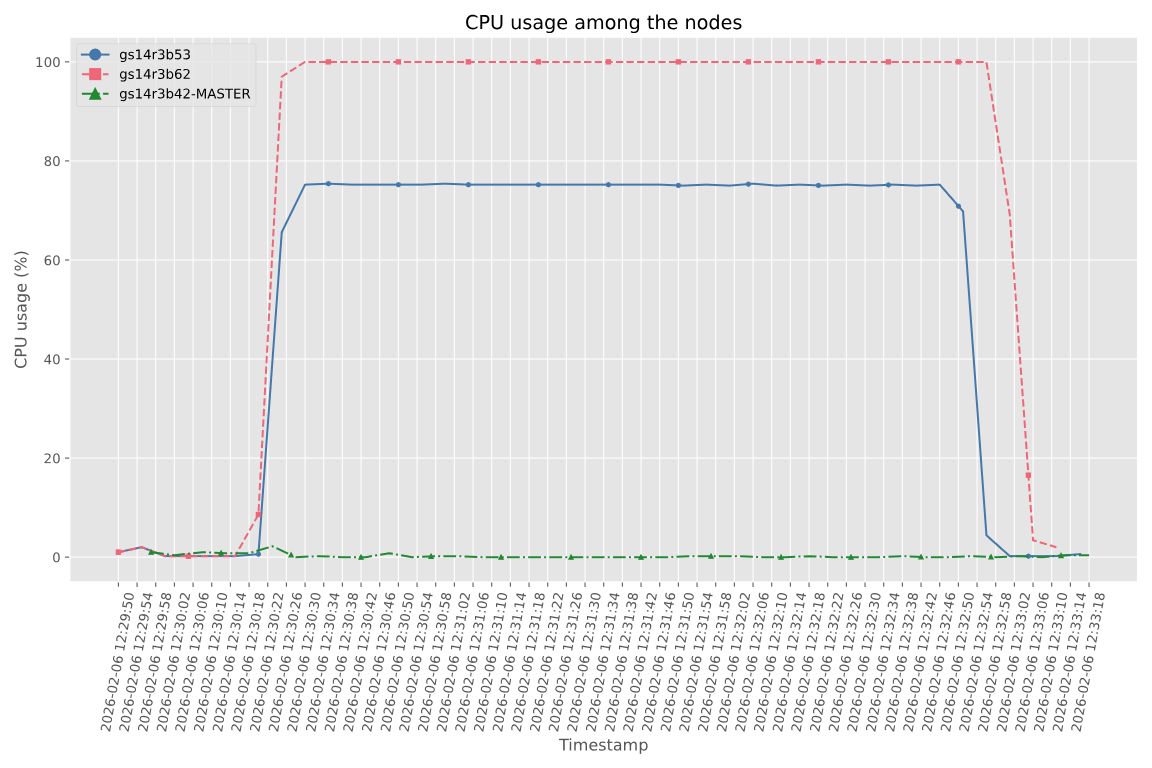
Figure 46 CPU usage plot
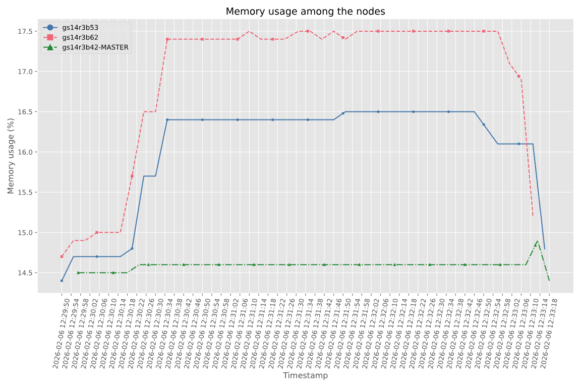
Figure 47 Memory usage plot